

Causal Inference in Practice: Geo-Experiments vs. Synthetic Control
Traditional online A/B testing often breaks down in retail, marketing, and pharma because interventions are deployed at the store, region, market, or territory level rather than at the individual level. A retailer cannot show two shelf prices to two shoppers in the same aisle; a marketing team buys media at the DMA (Designated Market Area) level, where exposure is only partly controllable; a pharma team assigns field-force coverage by physician territory, not by patient.
Once individual randomization is off the table, causal inference becomes a design problem shaped by clusters, spillovers, and credible counterfactuals. Geo-experiments, the Synthetic Control Method (SCM), and Difference-in-Differences (DiD) are the most practical tools here.
The Challenge of Physical A/B Testing
Digital A/B testing needs clean user-level assignment and fast, well-measured outcomes. Offline interventions rarely offer these: pricing, promotion, media spend, and field-force allocation are applied to aggregate units — stores, cities, regions, or physician territories.
That changes the statistical problem. Assignment becomes a cluster-level decision constrained by operations, regulation, and local market structure. The biggest threats are interference and contamination: cross-border shopping biases a price test when customers shift from treated to nearby control stores; advertising spillovers reach control markets through commuting or overlapping broadcast areas; a control region may inadvertently receive treatment through a national campaign or a shared field team. Small samples compound the problem; market outcomes are noisy, serially correlated, and shaped by holidays, weather, and stockouts.
Applied teams therefore need cluster-level or panel-based designs — geo-experiments, SCM, or DiD.
Methodological Comparison: Geo-Experiments vs. SCM
The choice usually comes down to one question: can you randomize treatment at the level where the decision is made? If yes, a geo-experiment is usually cleanest; if not, SCM beats a naive before-and-after comparison.
Geo-experiments: design logic and trade-offs
A geo-experiment assigns treatment across regions, stores, or territories, with comparable geos randomized into treatment and control. When assignment is independent of potential outcomes, post-treatment differences can be attributed to the intervention, provided the design prevents contamination — stronger internal validity than an observational design offers. The limitations are practical: expense, low power when geos are few, and vulnerability to spillovers.
Synthetic Control Method: construction and credibility
SCM is useful when a treated unit cannot be randomized and the analyst needs a credible counterfactual. It constructs a weighted combination of untreated units — the donor pool — reproducing the treated unit's pre-treatment path; the post-treatment gap versus this synthetic counterpart is the estimated effect.
Pre-treatment fit is the center of gravity: if the synthetic unit does not resemble the treated one before the intervention, it is hard to argue it captures the counterfactual afterward. Donor quality matters as much as model form — the pool should contain comparable untreated units under similar demand and competitive forces. Unlike DiD, SCM does not depend on raw average parallel trends; it matches on pre-treatment trajectories and, indirectly, on the latent factors driving outcomes. It works best with one or a few treated units and a long pre-treatment history.
Side-by-side decision framework
| Criterion | Geo-experiment | Synthetic Control Method |
|---|---|---|
| Identification | Randomized or quasi-randomized assignment across clusters | Weighted counterfactual built from untreated donor units |
| Best suited for | Multiple treated and control geos | One or a few treated units |
| Data needs | Clustered panel; moderate history helps | Long pre-period and rich donor pool are critical |
| Key assumptions | Valid assignment, SUTVA, limited contamination | No interference, strong pre-treatment fit, stable relationships |
| Inference | Clustered standard errors, randomization inference | Placebo tests and donor-pool sensitivity checks |
| Main risk | Spillovers, low power, high operational cost | Poor pre-period fit, donor dependence, fragile inference |
The practical rule: randomize geos when you can; when treatment is non-randomized and concentrated in one market, SCM beats a naive comparison. Newer variants such as augmented SCM and Synthetic DiD help in complex settings but do not remove the need for credible untreated comparisons.
Checking Assumptions: SUTVA and Parallel Trends
Method choice matters, but assumptions matter more. Design failures come from spillovers, anticipation, or poor counterfactuals rather than from regression syntax.
SUTVA (Stable Unit Treatment Value Assumption) has two parts: one unit's outcome should not depend on another unit's treatment, and the treatment must be well defined. At the geo level this is fragile — markets are porous and customers travel, so shoppers may react to higher prices in a treated store by visiting a nearby control store, biasing estimates in either direction. Mitigation starts before modeling: geographic buffers, excluded border markets, and less connected clusters often matter more than the specification.
For DiD, the identifying assumption is parallel trends: absent treatment, treated and control units would have experienced similar outcome changes, not identical levels. SCM substitutes pre-treatment fit for that comparison. In both cases, analysts should check for no anticipation, stable sample composition, and no confounding shocks. An event-study plot is the standard diagnostic, showing whether units were already diverging before treatment and how effects evolve after rollout.
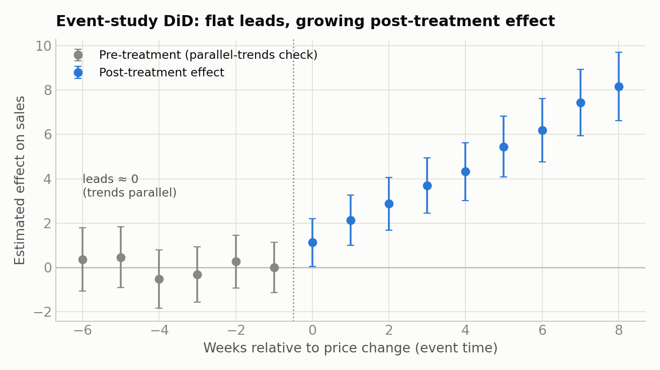
Figure 1. Event-study DiD. Pre-treatment coefficients sit near zero (evidence for parallel trends); post-treatment effects grow after the price change.
Clustered standard errors are usually needed because observations within a store are correlated over time; with few clusters, permutation- or placebo-based inference is preferable. In SCM, credibility improves when results hold across donor-pool definitions.
Practical Use Case: Price Optimization for a Physical Retail Pilot
A recent Grid Dynamics engagement makes the trade-offs concrete. A large Latin American grocery retailer had begun rolling out electronic shelf labels, which made frequent price changes feasible, and engaged the team to build a price-optimization engine setting a daily margin-maximizing price for each store-by-SKU pair under inventory and business constraints. The pilot covered ten product categories across three stores of different sizes.
Three stores is the crux. That is far too few for a randomized geo-experiment, and the stores were pre-selected by the business, so random assignment was never available. Store-level A/B testing was also unsuitable: a posted price applies to everyone in the store, and no two physical stores are truly comparable. The design moved to a Difference-in-Differences with Synthetic Control approach — build, for each treated store, a synthetic counterpart from untreated stores whose pre-treatment sales tracked it closely, then read the effect off the post-go-live gap.
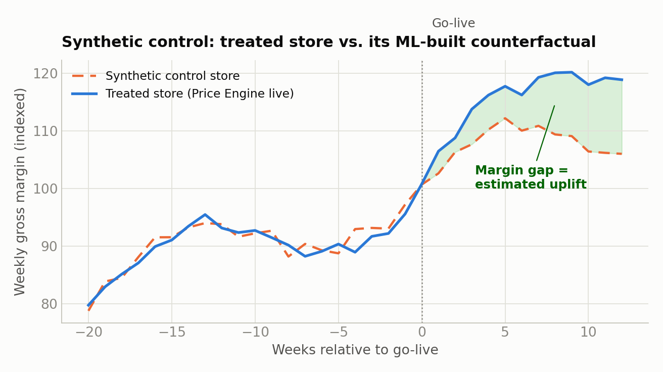
Figure 2. The treated store and its synthetic counterfactual track closely before go-live; the shaded post-go-live gap is the estimated margin uplift.
Two details proved decisive. Counterfactual selection was its own analysis: donor stores were screened on pre-period parallel trends before the synthetic weights were fixed, and several libraries (CausalImpact, causalpy, and dedicated synthetic-control packages) were compared first. Results were reported as ranges — point estimates with confidence intervals and explicit best- and worst-case scenarios — so stakeholders read the uplift as a distribution, not a single number. Pairing the synthetic control with a LightGBM demand forecaster also enabled a pricing-engine simulator, initially out of scope but central to tuning before deployment.
For a single treated unit, credibility rests on placebo testing: apply the same procedure to untreated donor stores and check whether similarly large effects appear where no treatment occurred. If they do not, this provides evidence that the treated store genuinely stands apart.
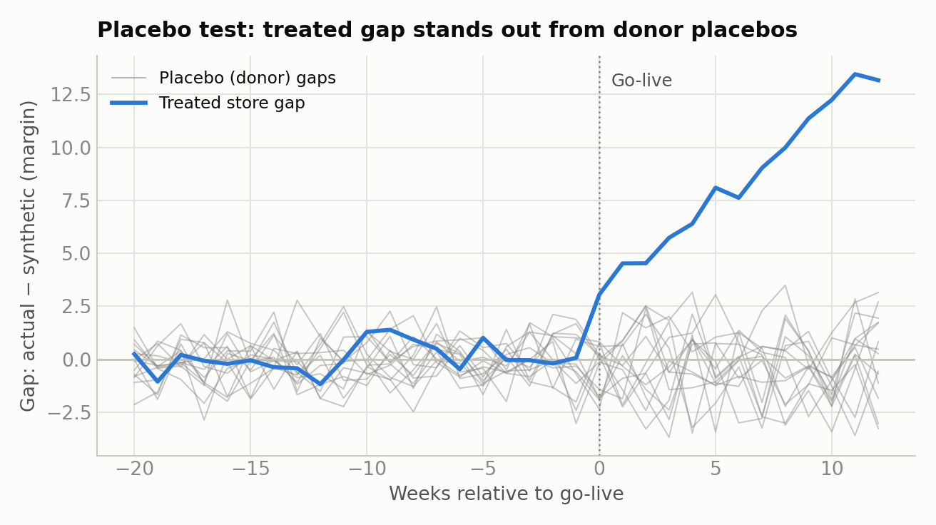
Figure 3. Placebo test. The treated store's gap (bold) separates from the donor placebo distribution (thin) after go-live — the basis for inference with a single treated unit.
Across the three pilot stores, the live test cut demand-forecast error by roughly 66% against the retailer's previous model and produced up to a 20% margin increase depending on the store, at an infrastructure cost near $100 per month.
Where randomization and comparable controls are available, the problem reduces to a standard DiD — say, a retailer raising prices in 40 pilot stores while 120 hold prices. A two-way fixed-effects model absorbs store- and week-level variation, and the treated_store × post interaction captures the average incremental effect.
import pandas as pd
import statsmodels.formula.api as smf

# df columns:
# store_id: unique store identifier
# week: time period identifier
# sales: outcome, e.g. weekly category sales
# treated_store: 1 for pilot stores, 0 for control stores
# post: 1 after the price change, 0 before

model = smf.ols(
    "sales ~ treated_store * post + C(store_id) + C(week)",
    data=df
).fit(
    cov_type="cluster",
    cov_kwds={"groups": df["store_id"]}
)

print(model.summary())

did_effect = model.params["treated_store:post"]
print(f"Estimated DiD effect on sales: {did_effect:.3f}")
The coefficient on treated_store:post is the estimated average incremental effect, conditional on store and week fixed effects. Clustering by store matters because weekly observations within a store are correlated. When adoption is staggered and effects vary over time, two-way fixed-effects estimates should be interpreted with care and heterogeneity-aware estimators considered.
Conclusion and Key Takeaways
Geo-experiments are the first choice when clean randomization across geos is feasible. SCM is more credible than a simple observational comparison when treatment is non-randomized and concentrated in one or a few units, though its value depends on donor quality and pre-treatment fit. DiD remains practical and scalable for many store-, region-, and market-level decisions.
The pilot above shows the pattern: with three pre-selected stores, neither randomization nor classic A/B testing applied, and a synthetic-control design supplied the counterfactual behind a credible margin estimate. The decision lens stays simple — randomize when possible, use SCM for a few treated units with strong donor pools, and use DiD for multi-store rollouts with careful validation. Causal inference is a design problem first and a modeling problem second.
References
- Abadie, A., Diamond, A., & Hainmueller, J. (2010). Synthetic control methods for comparative case studies. Journal of the American Statistical Association, 105(490), 493–505. https://doi.org/10.1198/jasa.2009.ap08746
- Abadie, A., & Gardeazabal, J. (2003). The economic costs of conflict: A case study of the Basque Country. American Economic Review, 93(1), 113–132. https://doi.org/10.1257/000282803321455188
- Bertrand, M., Duflo, E., & Mullainathan, S. (2004). How much should we trust differences-in-differences estimates? Quarterly Journal of Economics, 119(1), 249–275. https://doi.org/10.1162/003355304772839588
- Rubin, D. B. (1974). Estimating causal effects of treatments in randomized and nonrandomized studies. Journal of Educational Psychology, 66(5), 688–701. https://doi.org/10.1037/h0037350
- Vaver, J., & Koehler, J. (2011). Measuring ad effectiveness using geo experiments. Google Research. https://research.google/pubs/measuring-ad-effectiveness-using-geo-experiments/
- Brodersen, K. H., Gallusser, F., Koehler, J., Remy, N., & Scott, S. L. (2015). Inferring causal impact using Bayesian structural time-series models. Annals of Applied Statistics, 9(1), 247–274. https://doi.org/10.1214/14-AOAS788
- Arkhangelsky, D., Athey, S., Hirshberg, D. A., Imbens, G. W., & Wager, S. (2021). Synthetic difference-in-differences. American Economic Review, 111(12), 4088–4118. https://doi.org/10.1257/aer.20190159
- Ben-Michael, E., Feller, A., & Rothstein, J. (2021). The augmented synthetic control method. Journal of the American Statistical Association, 116(536), 1789–1803. https://doi.org/10.1080/01621459.2021.1929245
- Callaway, B., & Sant'Anna, P. H. C. (2021). Difference-in-differences with multiple time periods. Journal of Econometrics, 225(2), 200–230. https://doi.org/10.1016/j.jeconom.2020.12.001
- Roth, J., Sant'Anna, P. H. C., Bilinski, A., & Poe, J. (2023). What's trending in difference-in-differences? A synthesis of the recent econometrics literature. Journal of Econometrics, 235(2), 2218–2244. https://doi.org/10.1016/j.jeconom.2023.03.008
- Facure, M. (2022). Causal Inference for the Brave and True. https://matheusfacure.github.io/python-causality-handbook/landing-page.html